Analysis of Trends in Temperature
Introduction
There exists a growing body of scientific research aimed at assessing the causes and effects of climate change and global warming in the world. While the causes are, today, well-established, it is important to estimate the temperature trends on a regional scale in order to correctly assess the effects on the local ecosystems and improve policymaking. The assignment focused on the Netherlands, a country known for its vulnerability to the rising sea levels and it is highly probable that a sizable increase in temperature would influence the likelihood of such phenomenon. The scope of our investigation was limited to 3 cities: De Bilt, Eelde, and Maastricht over the span of a century (1907-2023) and aimed to estimate the presence of a long-term trend in the daily, monthly, and annual temperature data provided by the course coordinator, Prof. Stephen Smeekes.
Data
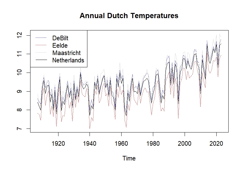
Figure 1: Annual Dutch Temperatures
The temperature data for the three cities can be thought of as the realization of three time series processes. Since the analysis is concerned with the Netherlands, those series are more useful when aggregated. We have, thus, generated a new series for the Netherlands by averaging the three processes.
The time series processes still seem quite “rocky”, we decided to smooth the data by computing the cumulative ten-year average for each point as follows:
tenyear <- function(data) {
  n <- length(data) - 9
  averages <- rep(0, n)
  for(i in 1:n) {
    subset <- data[i:(i+9)]
    averages[i] <- mean(subset)
  }
  return(averages)
}
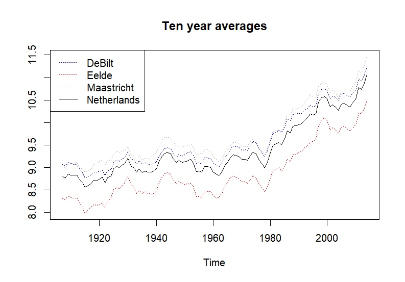
Figure 2: Smoothed Dutch Temperatures
The series appear smoother than in the original plot. What appeared to be a positive trend in Figure $1$, seems to confirmed in the smoothed plot. Despite some slight differences in average temperatures of around $1$ °C, the series fluctuate in the same way. This is, however, unsurprising due to the small size of the country.
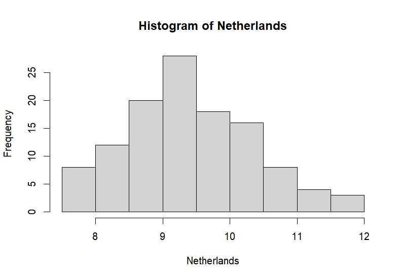
Figure 3: Histogram of Netherlands
The paper relies exclusively on the use of ordinary least squares regression to estimate the trend in the temperature data. This method is sensible to the presence of outliers which tends to bias the estimated coefficients. Their presence can be investigated using a histogram. The plot only shows the possibility of right-skewness which could hint towards an upward trend in the dataThe skewness indicates that above-average temperatures are less common than those below while being more likely to deviate further from the mean..
Measuring the statistical significance of the possible trend requires us to make some distributional assumption. Given the limited sample (of $117$ observations), it makes sense to assume that the data is generated from a $\text{T}$-distribution with $116$ degrees of freedom. To simplify the analysis, the data is assumed to be independent and identically distributed (i.i.d). This may be unlikely to hold due to the nature of the data.
Code
Note that for this assignment, we were required to code most of the statistical methods we wished to use ourselves. Our output is often slightly different from the standard methods due to (lack of) rounding.
Research
Annual data
The first model we investigate is the regression of temperature of the Netherlands over a trend.
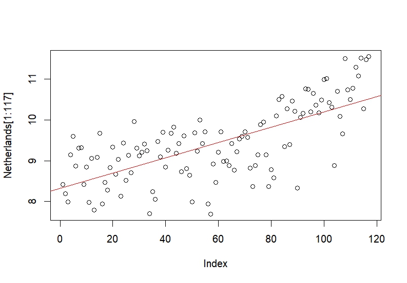
Figure 4: Trend of the Netherlands
The output of the regression shows that there is a trend in the data, and the reported T-value is significant at both the $5\%$ and $1\%$ significance levels. The null hypothesis of the test was $H_{0}: \beta \leq 0$ vs. $H_{1}: \beta \gt 0$. We conducted a right-tailed test such that if the p-value is small enough, we can be confident about the presence of a positve trend.
Model $1$:
| Parameter | Estimate | Std. Error | T-value | P-value |
|---|---|---|---|---|
| Intercpt | 8.31828 | NA |
NA |
NA |
| Slope | 0.01874 | 0.00182 | 10.29 | 2.44e-18 |
The $95\%$ confidence interval for the slope coefficient is $[0.0157; \infty)$. The fact that $0$ lies outside of the $95\%$ confidence interval is an other indicator that the null hypothesis should be rejected. This model, however, is not very satisfactory. It seems that the trend in the last $50$ years of is greate than the trend earlier in the sample. For this reason, we created a sub-sample including all the data after $1974$ and regressed it on a trend variable.
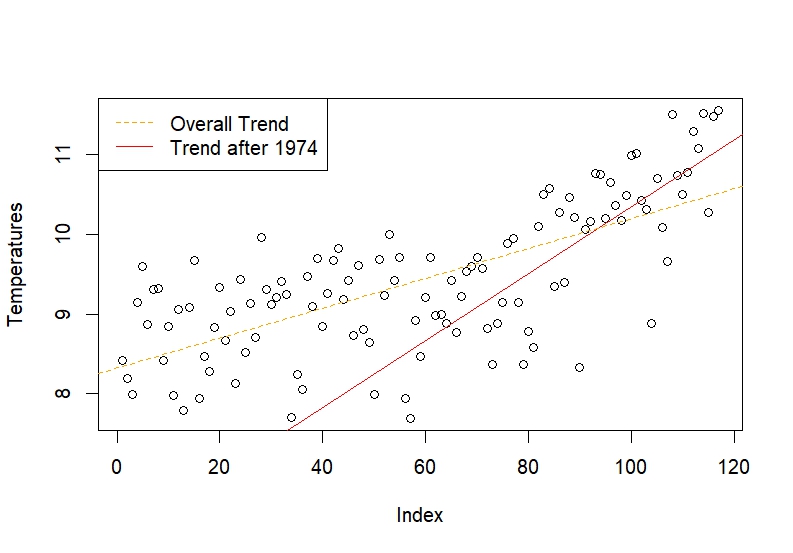
Figure 5: Trends of the Netherlands
Model $2$:
| Parameter | Estimate | Std. Error | T-value | P-value |
|---|---|---|---|---|
| Intercpt | 9.00651 | NA |
NA |
NA |
| Slope | 0.04192 | 0.00618 | 6.783 | 7.19e-09 |
The trend is significant and the $95\%$ confidence interval $[0.0316; \infty)$ indicates that the upward trend has become steeper in the last decades since the trend found in Model $1$ lies outside the interval.
Extension to Monthly data
While the presence of an upward trend was already established in the previous section, now we aim to get a more precise estimate for that trend. A model equivalent to Model $1$ is ran on the monthly dataset.
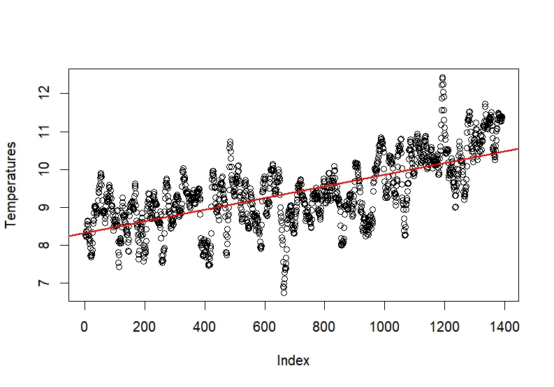
Figure 6: Monthly trends of the Netherlands
Model $3$:
| Parameter | Estimate | Std. Error | T-value | P-value |
|---|---|---|---|---|
| Intercpt | 8.31391 | NA |
NA |
NA |
| Slope | 0.00154 | 4.54e-05 | 33.83 | 7.56e-184 |
The output of Model $3$ shows that the trend is significant. We transformed the monthly trend into an annual trend to test the likelihood of whether the trend in Model $1$ is greater than the implied annual trend of Model $3$. The t-test is a right-tailed test set up as follows:
Hypothesis Testing:
-----------------------------------
Null: the slope is less or equal to 0.01848
Alt: the slope is greater than 0.01848

           T value P-value
    Slope: 0.1455583 0.4422613
The output of the t-test implies that we fail to reject the null hypothesis. The true trend of the whole process could be smaller than $0.01848$. However, we cannot reach this conclusion with confidence. This value can be thought of as an “unofficial” upper bound that could be interesting to keep in mind.
The Bootstrap
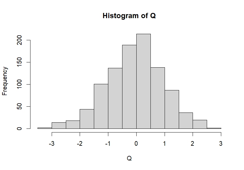
Figure 7: Bootstrap distribution of the Netherlands
The histogram shows the distribution of the Bootstrap T-statistics.
The Bootstrap is a statistical technique developed by Bradley Efron. Essentially, the original sample is randomly resampled with replacement a large number of times to improve the estimates of our coefficients. The speed of our computers led us to chose a replication size of $1000$ for the bootstrap. In Figure $7$, we see that the distribution is less skewed than before. The distribution seems to be converging to a Normal distribution. Since the standard deviation of the population model is unknown, we assume a T-distribution.
We construct a tow-tailed $95\%$ confidence interval around the mean $[9.262; 9.585]$, and can reasonably expect the population mean to lie within these bounds. Earlier, we considered the subsample starting in $1974$, the bootstrap confidence interval for the mean of this subsample is $[9.825; 10.294]$. This slightly wider interval indicates that the mean of the sample has shifted upwards. Also, given that there is no overlap between the bootstrap confidence interval for the full sample and that for the “after 1974” subsample, it can be concluded the means of those samples are significantly different from one another. This goes in line with previously drawn conclusions.
Conclusion
The evidence of human-made global warming is overwhelming in the scientific litterature. In this paper, we aimed to asses the statistical significance of the increase in temperature in the last century. The trend found in Model $1$ was shown to be significant and tells us that, over the full sample, the temperature has increased by roughly $2$ °C in the Netherlands. Further, analysis has allowed us to concluded that the increase in temperature is more pronunced in recent times than earlier in the sample. These results have some alarming implications for the Netherlands and should hopefully put more pressure on policymakers and large organizations to implement measures to tackle the issue of global warming, and reduce global $CO_{2}$ emissions.